词向量(词嵌入，Word Embedding)已经比较熟悉了，但还是整体梳理一下比较好。不再详细介绍它的背景和简介，而是将能想到的细节进行整理说明。

语言模型

语言模型的任务定义:对于语言序列$w_1,w_2,w_3,…,w_n$,语言模型就是计算该序列的概率，即$P(w_1,w_2,w_3,….,w_n)$。从机器学习角度来看，语言模型就是对语句的概率分布进行建模。简单来说，可以用语言模型来比较两个语句哪个更加正常,如 $P(\text{I am Light}) > P(\text{Light I am})$。由概率公式可得：
$$P(w_1,w_2,w_3,….,w_n) = P(w_1)\cdot P(w_2 | w_1) \cdot P(w_3 |w_1, w_2)\cdot \ … \ P(w_n|w_1,w_2,…w_{n-1})$$

在统计学领域，语言模型通常是使用n-gram语言模型，即使用size为n的window对序列切分建模，这里不再展开。

2003年，Bengio发表了神经网络语言模型(NNLM)论文[1]，其网络结构如下图所示：

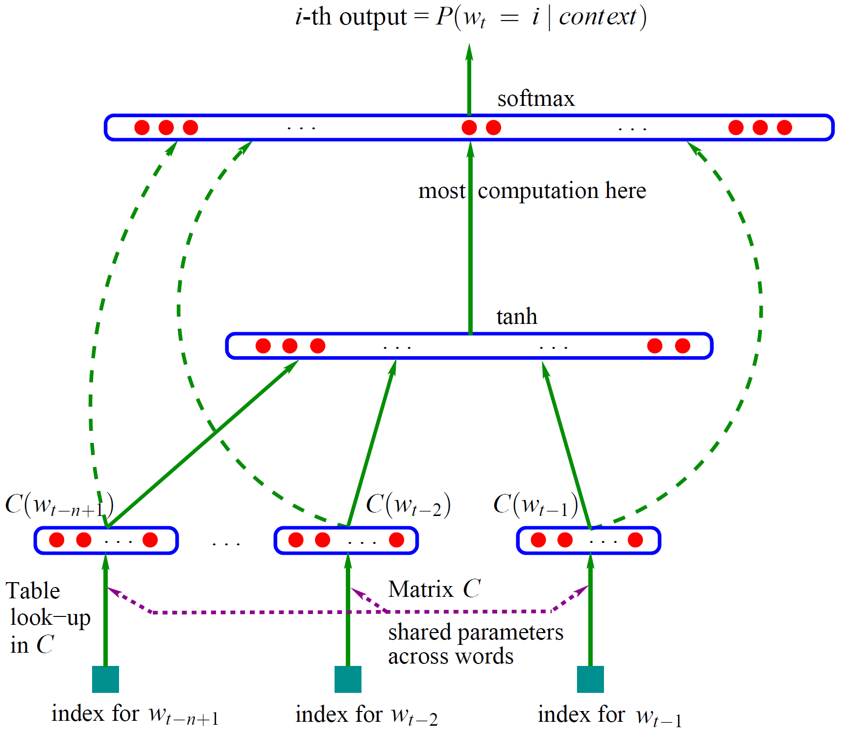
NNLM包含输入层，隐层，输出层三层神经网络，首先来看输入层，将单词$w_t$的上文(前n个单词)使用one-hot形式表示，并乘以矩阵$C$(跟据one-hot形式可发现是查表操作)。然后将得到的向量拼接在一起得到 $[C(w_{t-n+1}), …C(W_{t-2}), C(W_{t-1})]$ ，其作为隐层的输入。隐层的激活函数为tanh。最后输出层使用Softmax进行词汇表 $V$ 上的分类。矩阵$C$初始是随机初始化的，通过NNLM任务发现，学习后的矩阵$C$是一个密集且包含语义的词向量矩阵。通过one-hot进行相乘可得到每个单词对应的词向量。

one-hot向量长度为词汇表$V$维向量，嵌入维度m可自行设定。在cs224n课程中，矩阵$C$及隐层权重$W$都用来表示词嵌入，后者被成为上下文向量。在吴恩达课程中，嵌入矩阵即为矩阵$C$。

通过NNLM任务，作为副产品的词向量效果良好，进而将其发扬光大。

Word2vec

Word Embedding的常用技术：word2vec主要任务目标就是为了训练得到词向量，而不再是NNLM的任务。word2vec包含两个模型CBOW，Skip-gram。word2vec是由两篇论文[2][3]完成的，第一篇论文提出了两个模型，第二篇论文提出了两个训练技巧，使训练更加有效可行。

模型细节

@word2vec模型
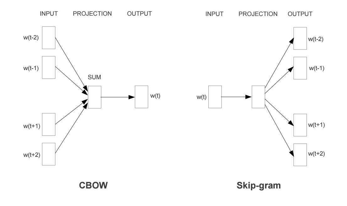
CBOW模型是将中心词的上下文作为输入来进行预测，而Skip-gram是根据中心词来预测其上下文单词。二者其实差不多。现在以Skip-gram为例来介绍下细节[4]。

我们想要训练一个神经网络，抽取语句中的一个中间词来作为输入单词，然后随机选择’临近’的一个单词(‘临近’即超参数window size，通常选择5，即中心词前后各五个单词)。网络的输出概率应该为那些比较相关的单词。比如输入单词为”Soviet”,那输出结果 “Union” 和 “Russia”的概率应该高于其它不相关的单词。

@skip-gram的训练样本
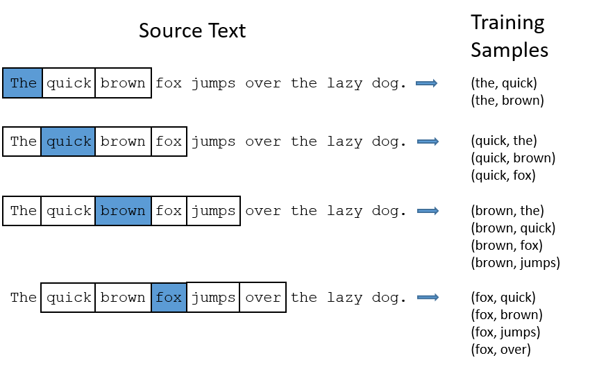
网络应该能从单词组的共现次数上学习到统计信息。比如词组(“Soviet”, “Union”)出现是高于(“Soviet”, “Sasquatch”)，当网络在训练完成后，输入”Soviet”得到的结果中，”Union” 或 “Russia” 的概率应高于 “Sqsquatch”。

@网络结构

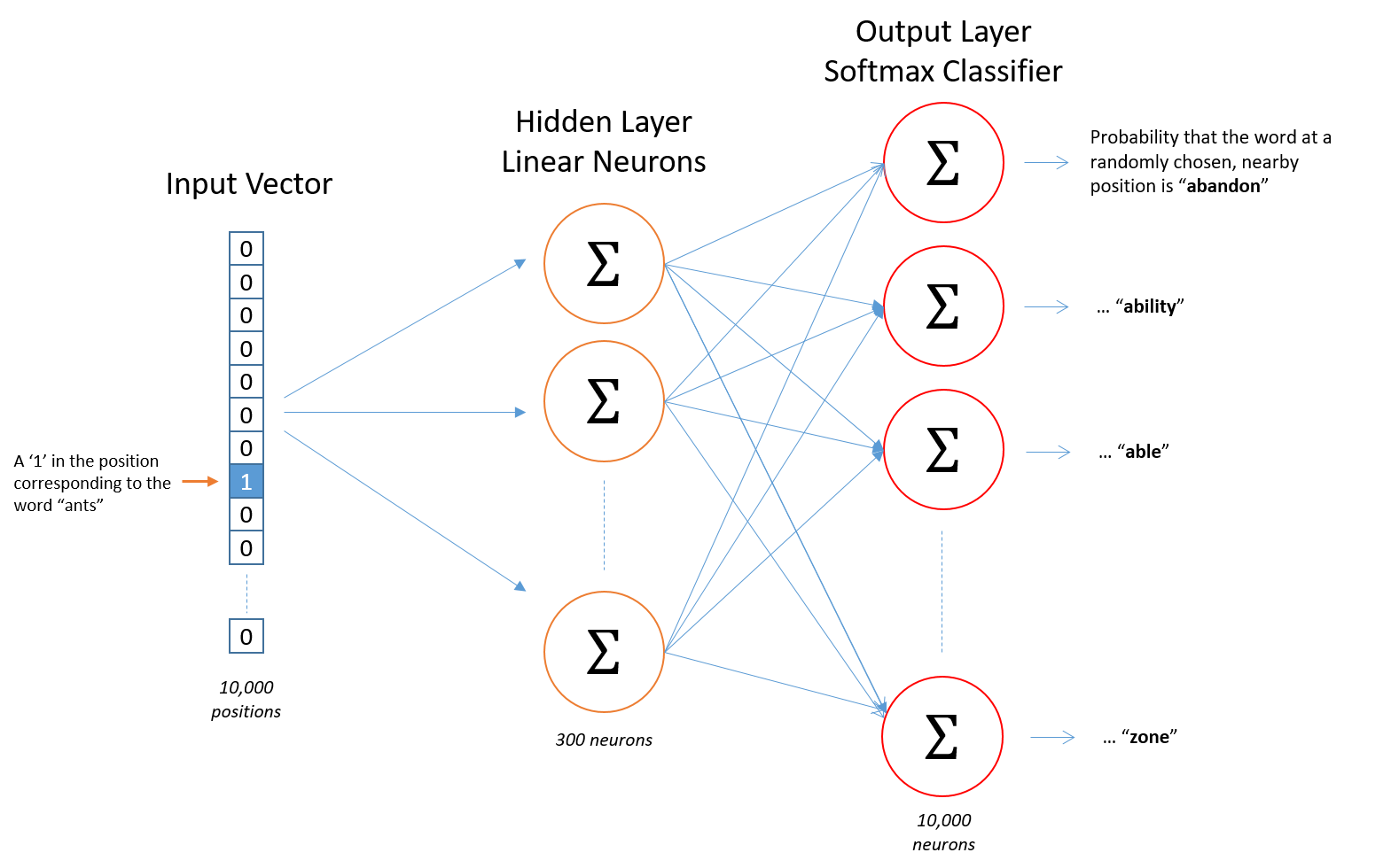
加入词汇表长度为10000，首先使用one-hot形式表示每一个单词，经过隐层300个神经元计算，最后使用Softmax层对单词概率输出。每一对单词组，前者作为x输入，后者作为y标签。

隐层细节

假如我们想要学习的词向量维度为300，则需要将隐层的神经元个数设置为300(300是Google在其发布的训练模型中使用的维度，可调)。

隐层的权重矩阵就是词向量，我们模型学习到的就是隐层的权重矩阵。

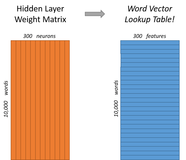
之所以这样，来看一下one-hot输入后与隐层的计算就明白了。

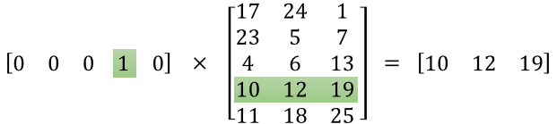
当使用One-hot去乘以矩阵的时候，会将某一行选择出来，即查表操作，所以权重矩阵是所有词向量组成的列表。

输出层细节

Softmax细节不再阐述，其能将输出进行概率归一化。

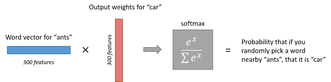
注意，神经网络并没有学习到输出相对于输入的偏移量。比如，在我们的语料库中，’York’每次前面都有’New’这个单词，所以，从训练数据角度来讲，’New’与’York’附近的概率为100%，但在’York’附近随机取10个单词，那概率就不再是100%了。

问题

假如使用词向量维度为300，词汇量为10000个单词，那么神经网络输入层与隐层，隐层与输出层的参数量会达到惊人的300x10000=300万！训练如词庞大的神经网络需要庞大的数据量，还要避免过拟合。因此，Google在其第二篇论文中说明了训练的trick，其创新点如下：

将常用词对或短语视为模型中的单个”word”。
对频繁的词进行子采样以减少训练样例的数量。
在损失函数中使用”负采样(Negative Sampling)”的技术，使每个训练样本仅更新模型权重的一小部分。

子采样和负采样技术不仅降低了计算量，还提升了词向量的效果。

对频繁词子采样

@'the'问题
在以上例子中，可以看到频繁单词’the’的两个问题:

对于单词对(‘fox’,’the’)，其对单词’fox’的语义表达并没有什么有效帮助，’the’在每个单词的上下文中出现都非常频繁。
预料中有很多单词对(‘the’,…)，我们应更好的学习单词’the’

Word2vec使用子采样技术来解决以上问题，根据单词的频次来削减该单词的采样率。以window size为10为例子，我们删除’the’：

当我们训练其余单词时候，’the’不会出现在他们的上下文中。
当中心词为’the’时，训练样本数量少于10。

采样率(Sampling rate)
使用 $w_i$来表示单词，$z(w_i)$来表示单词的频次。采样率是一个参数，默认值为0.001。$P(w_i)$ 表示单词保留的概率：
$$P(w_i)=(\sqrt{\frac{z(w_i)}{0.001}} +1) \cdot \frac{0.001}{z(w_i)}$$
该函数的图像为：

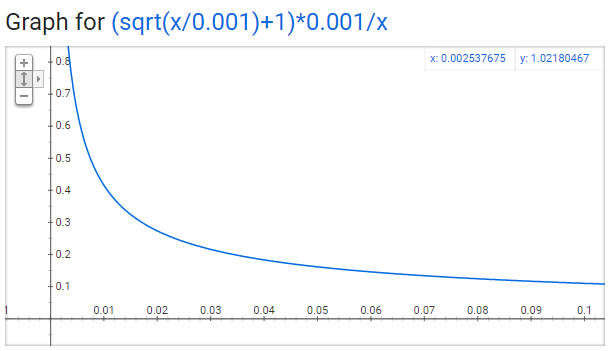
可以发现随着频次x的增加，其保留的概率越低。关于此函数有三个点需要注意：

$P(w_i) = 1.0$(100%保留)，对应的 $z(w_i)<=0.0026$。(表示词频大于0.0026的单词才会进行子采样)
$P(w_i) = 0.5$(50%保留)，对应的 $z(w_i)=0.00746$。
$P(w_i) = 0.033$(3.3%保留)，对应的 $z(w_i)=1.0$。(不可能)

负采样(Negative Sampling)

训练一个网络是说，计算训练样本然后轻微调整所有的神经元权重来提高准确率。换句话说，每一个训练样本都需要更新所有神经网络的权重。

就像如上所说，当词汇表特别大的时候，如此多的神经网络参数在如此大的数据量下，每次都要进行权重更新，负担很大。

在每个样本训练时，只修改部分的网络参数，负采样是通过这种方式来解决这个问题的。

当我们的神经网络训练到单词组(‘fox’, ‘quick’)时候，得到的输出或label都是一个one-hot向量，也就是说，在表示’quick’的位置数值为1，其它全为0。

负采样是随机选择较小数量的’负(Negative)’单词(比如5个)，来做参数更新。这里的’负’表示的是网络输出向量种位置为0表示的单词。当然，’正(Positive)’(即正确单词’quick’)权重也会更新。

论文中表述，小数量级上采用5-20，大数据集使用2-5个单词。

我们的模型权重矩阵为300x10000，更新的单词为5个’负’词和一个’正’词，共计1800个参数，这是输出层全部3M参数的0.06%！！

负采样的选取是和频次相关的，频次越高，负采样的概率越大：
$$P(w_i) = \frac{f(w_i)^{3/4}}{\sum_{j=0}^n(f(w_j)^{3/4})}$$
论文选择0.75作为指数是因为实验效果好。C语言实现的代码很有意思：首先用索引值填充多次填充词汇表中的每个单词，单词索引出现的次数为$P(w_i) * \text{table_size}$。然后负采样只需要生成一个1到100M的整数，并用于索引表中数据。由于概率高的单词在表中出现的次数多，很可能会选择这些词。

分层Softmax

Skip-gram 代码实现

Skip-gram的实现有多种方式，比如很多软件包(gsim)已经收录了，可以直接调用。Skip-gram模型并不复杂，网络仅有一个隐层，使用Keras实现也非常简单，但是自己手写实现更更好理解一些。这里讲下自己的实现。主要参考Tensorflow word2vec模型,该实现封装数据集及推理(analogy)等内容，但对神经网络的定义、负采样、NCE损失函数等内容的，虽然并不都是完全底层实现，但对深入理解还是很有帮助的。数据集采用的是20newsgroups，这个数据集有个博士处理后的版本(去除了停用词the等)。20newsgroups数据还是比较粗糙的，整个实现比较随意，源jupyter及训练数据也就没有上传github,但对模型理解还是有帮助的。

加载数据

def load_data():
    """加载数据"""
    
    newsgroup = fetch_20newsgroups(data_home='./ataset/20newgroups/',
                          subset='all',
                          remove=('headers', 'footers', 'quotes'))
    
    corpus = ''.join(newsgroup.data).lower().split()
    counter_corpus = Counter(corpus)

    words_count = sorted(counter_corpus.items(), key=lambda kv:kv[1], reverse=True)
    stop_words = '? ! @ # $ % ^ & * ( ) [ ] { } > < = - + ~ ` --- (i (or / ; ;\' $1 |> \
                    --------- -------------------------------------------------------------------------- \
                    ========================= \
                    0 1 2 3 4 5 6 7 8 9 13 15 30 24 20 "a" tk> 95 45'
    
    index = 0
    vocab_words, vocab, reverse_vocab, vocab_count, vocab_freq,= [],{},{},{},{}
    for (k,v) in words_count:
        if k in stop_words.split() or v < 15: continue
        # 单词列表
        vocab_words.append(k)
        # 单词:id
        vocab[k] = index
        # id:单词
        reverse_vocab[index] = k
        # 单词:频次
        vocab_count[k] = v
        # 单词:频率
        vocab_freq[index] = v/len(corpus)
        index += 1

    print('字典长度:', len(vocab.keys()))
    print(vocab_words[:10])
    
    corpus_int = [vocab.get(word) for word in corpus]
    # 非字典词语占比
    print('非字典词语占比%.2f' % (corpus_int.count(None)/len(corpus_int)*100))
    
    samples = generate_samples(corpus_int, vocab, vocab_freq) # version2 实现子采样 传入原始语料(word list)而不是int
    print('样本数量:',len(samples))
    
    return samples, list(vocab_count.values()), vocab

使用子采样方式生成训练数据

def generate_samples(corpus, vocab, vocab_freq):
    """使用子采样生成数据"""
    LEN = len(corpus)
    rate = 0.001
    samples = []
    
    for i,center_word in enumerate(corpus):
        # 非词汇表词过滤
        if i-2<0 or i+2>LEN-1 \
            or center_word is None \
            or center_word == vocab['.']:
            continue
        else:
            condedate_words = [center_word, corpus[i-1], corpus[i-2], corpus[i+1], corpus[i+2]]
            condedate_words = [word for word in condedate_words if word is not None]
            freqs = np.array([vocab_freq[word] for word in condedate_words])
            p_keeps = (np.sqrt(freqs/rate) + 1) * rate / freqs
            p_keeps[p_keeps>1] = 1
            
            if  random.random() > p_keeps[0]: 
                # center_word 子采样
                # print('center_word %d 舍弃' % center_word)
                continue
            else:
                # target_word 子采样
                sampled_words = [(center_word, condedate_words[i+1]) for i,p in enumerate(p_keeps[1:]) if random.random()<p]
                samples.extend(sampled_words)
                
    return samples

子采样需要注意，论文中使用的采样公式与cs224n课程中不一样，但都可以实现，别忘记对数值进行截断，概率最大为1。

skip-gram 网络定义

emb_dim = 300
vocab_size = len(vocabulary)
batch_size = 128
num_samples = 5
epoches = 1000
top_n = 10
val_data = ['geometric', 'monitor', 'mouse', 'linux', 'microsoft', 
                           'engine', 'factory', 'storage', 'billion', 'article']


def forward(vocab, counts):
    """Build the graph for the forward pass."""
    
    examples = tf.placeholder(tf.int32, shape=[batch_size], name='input')
    labels = tf.placeholder(tf.int32, shape=[batch_size, 1], name='label')
    
    # Embedding Weight [vocab_size, emb_dim]
    init_width = 0.5 / emb_dim
    emb = tf.Variable(
        tf.random_uniform(
            [vocab_size, emb_dim], -init_width),
        name='emb')
    
    # Softmax Weight [vocab_size, emb_dim].Transposed.
    sm_w_t = tf.Variable(
        tf.zeros([vocab_size, emb_dim]),
        name='sm_w_t')
    
    # Softmax bias [vocab_size]
    sm_b = tf.Variable(tf.zeros([vocab_size]), name='sm_b')
    
    # NCE loss
    labels_matrix = tf.reshape(
        tf.cast(labels, dtype=tf.int64),
        [batch_size, 1])
    
    # Negative sampling
    sampled_ids, _, _ = (tf.nn.fixed_unigram_candidate_sampler(
        true_classes=labels_matrix,
        num_true=1,
        num_sampled=num_samples,
        unique=True,
        range_max=vocab_size,
        distortion=0.75,
        unigrams=counts))
    
    # Embeddings for examples: [batch_size, emb_dim]
    example_emb = tf.nn.embedding_lookup(emb, examples)
    
    # Weights for labels: [batch_size, emb_dim]
    # 不需要计算所有的logistic 仅计算正确单词的logistic进行更新
    true_w = tf.nn.embedding_lookup(sm_w_t, labels)
    true_b = tf.nn.embedding_lookup(sm_b, labels)
    
    # Weights for sampled ids: [num_sampled, emb_dim]
    sampled_w = tf.nn.embedding_lookup(sm_w_t, sampled_ids)
    # Biases for sampled ids: [num_sampled, 1]
    sampled_b = tf.nn.embedding_lookup(sm_b, sampled_ids)
    
    # True logits: [batch_size, 1]
    true_logits = tf.reduce_sum(tf.multiply(example_emb, true_w), 1) + true_b
    
    # Sampled logits: [batch_size, numsampled]
    sampled_b_vec = tf.reshape(sampled_b, [num_samples])
    sampled_logits = tf.matmul(example_emb, 
                               sampled_w, 
                               transpose_b=True) + sampled_b_vec
    
    # Similarity option
    norm = tf.sqrt(tf.reduce_sum(tf.square(emb), axis=1, keepdims=True))
    norm_emb = emb / norm
    
    
    val_int = tf.constant([vocab[word] for word in val_data], dtype=tf.int32)
    val_emb = tf.nn.embedding_lookup(norm_emb, val_int)
    similarity = tf.matmul(val_emb, tf.transpose(norm_emb))
    
    return examples, labels, true_logits, sampled_logits, similarity

def nec_loss(true_logits, sampled_logits):
    """Build the graph for the NCE loss."""

    # cross-entropy (logits, labels)
    true_xent = tf.nn.sigmoid_cross_entropy_with_logits(
        labels=tf.ones_like(true_logits), logits=true_logits)
    
    sampled_xent = tf.nn.sigmoid_cross_entropy_with_logits(
        labels=tf.zeros_like(sampled_logits), logits=sampled_logits)
    
    # NCE-loss is sum of the true and noise (sampled words)
    # contributions, average over the batch.
    nce_loss_tensor = (tf.reduce_sum(true_xent) + 
                       tf.reduce_sum(sampled_xent)) / batch_size
    
    return nce_loss_tensor

def optimize(loss):
    """Build the graph to optimize the loss function."""
    optimizer = tf.train.GradientDescentOptimizer(0.01).minimize(loss)
    return optimizer

def nearby():
    pass

def train(center_words, target_words, vocab, reverse_vocab, counts):
    """Build the graph for the full model."""
    
    tf.reset_default_graph()
    
    examples, labels, true_logits, sampled_logits, similarity = forward(vocab, counts)
    loss = nec_loss(true_logits, sampled_logits)
    optimizer = optimize(loss)
    
    saver = tf.train.Saver()
    with tf.Session() as sess:
        sess.run(tf.global_variables_initializer())
        
        batch_all = len(center_words) // batch_size
        print('Batch_all:', batch_all, 'Batch_size:', batch_size, 'Samples:', len(center_words))
        for epoch in range(epoches):
            for num in range(batch_all):
                x_batch = center_words[num*batch_size: batch_size*(num+1)]
                y_batch = target_words[num*batch_size: batch_size*(num+1)]

                y_batch = np.array(y_batch).reshape(-1, 1)

                _, l = sess.run([optimizer, loss], feed_dict={
                    examples : x_batch,
                    labels : y_batch
                })
                if num % 100 == 0:
                    print('Epoch:',epoch,' Iter', num, 'loss:', l)
                if num % 1000 == 0:
                    sim = similarity.eval()
                    for i,j in enumerate(val_data):
                        nearest_n = (-sim[i, :]).argsort()[1:top_n+1]
                        logg = 'Nearest to %s is :' % j
                        for ind,ner_int_word in enumerate(nearest_n):
                            nearest_word = reverse_vocab[ner_int_word]
                            logg = '%s  %s'%(logg,nearest_word)
                        print(logg)
        
        save_path = saver.save(session, "./checkpoints/word2vec_model_20news.ckpt")

网络定义基本手写copy github官方模型，在这可以看到NCE loss是如何计算，一般理解负采样是在反向传播简化计算，其实也是直接在前向进行计算简化，这点比其它博文教程要好。

训练

训练就比较简单，直接上就行。

不过即使使用了子采样，the的中心词数据也在30W+,调参不如直接删除~ 用博士处理后的数据训练效果会好一些，但那个数据的分词也挺烂的~
1
2
3
4
5
6
samples,counts,vocabulary = load_data()
reverse_vocab = {v:k for k,v in vocabulary.items()}
center_words = [x for (x,y) in samples]
target_words = [y for (x,y) in samples]

train(center_words, target_words, vocabulary, reverse_vocab, list(counts))

总之，skip-gram的效果还是可以看到的。

参考

[1] A Neural Probabilistic Language Model
[2] Distributed Representations of Words and Phrases and their Compositionality
[3] Efficient Estimation of Word Representations in Vector Space
[4] cs224n: Word2Vec Tutorial - The Skip-Gram Model
[5] word2vec Parameter Learning Explained
[6] [Tensorflow word2vec模型]
[7] 20newsgroups数据集